Examples

Numerical Simulators

In this file, we choose a benchmark plant, CSTR shown in the following figure, controlled by a PID controller. Also, we define the bias sensor attack that subtracts 25K from the temperature sensor feedback starting from the ninth second. The detector identifies the attack at the 10th second, and triggers the recovery controllers. Baseline recovery controllers include (i) no recovery method (none), (ii) software-sensor-based recovery (ssr [1]_), (iii) linear-quadratic-regulator-based recovery (lqr [2]_), and (vi) data-predictive recovery (mpc [3]_).

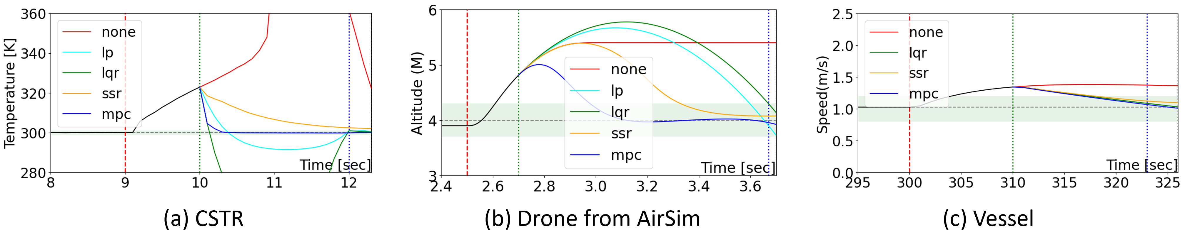
First, we aim to evaluate the recovery performance of different baseline recovery controllers. We only require modifying the configuration file rather than writing simulation code. In this file, we use three benchmark plants, CSTR, quadrotor and Vessel, controlled by a PID controller. Also, we define the bias sensor attack. The detector identifies the attack after the attack happends and triggers the recovery controllers. Baseline recovery controllers include (i) no recovery method (none), (ii) software-sensor-based recovery (ssr [1]_), (iii) linear-quadratic-regulator-based recovery (lqr [2]_), and (vi) data-predictive recovery (mpc [3]_).

The following figure plots the results from the simulator. From the curve, we can intuitively analyze the recovery performance of each baseline recovery controller.

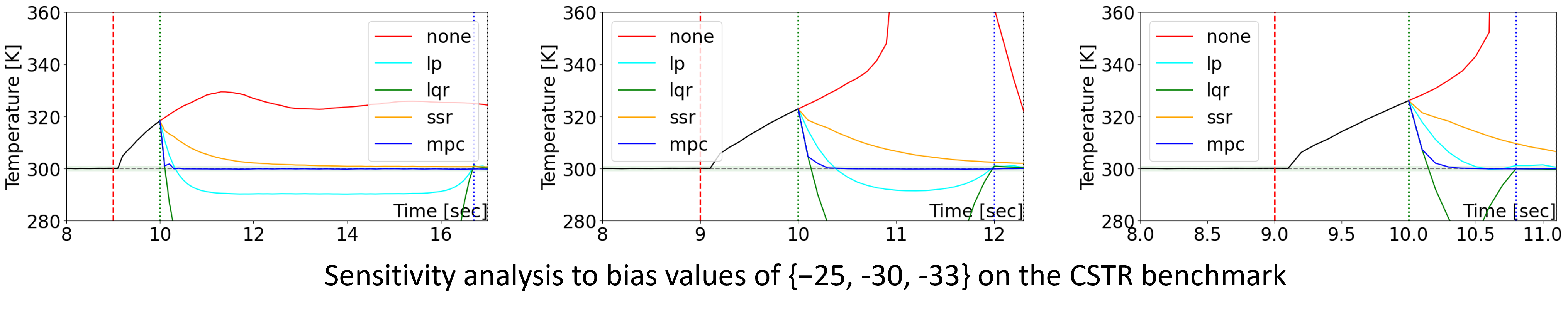
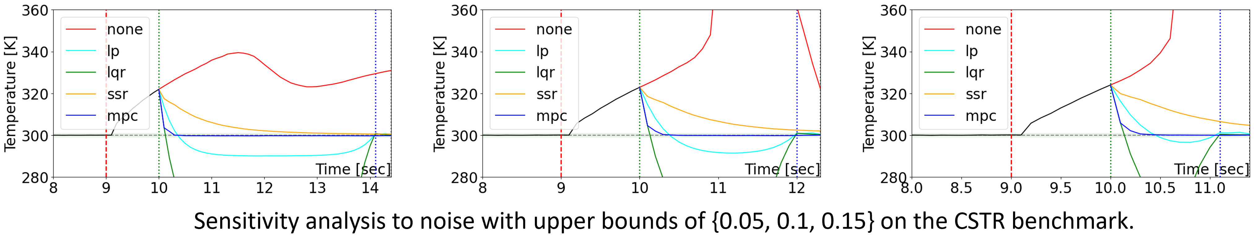
We conduct a sensitivity analysis by varying bias values and noise on the CSTR benchmark. The findings are displayed in the two figures below.

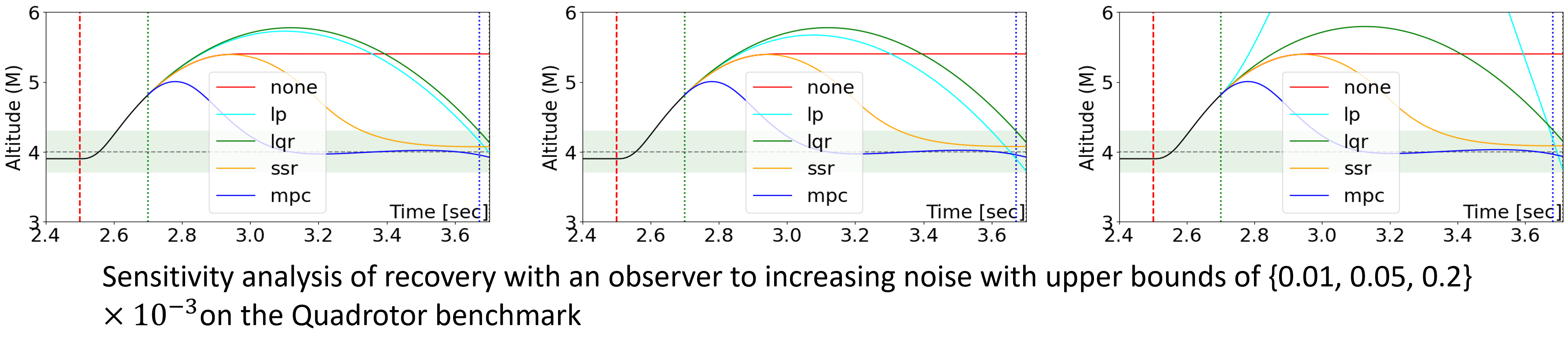
We also provide the sensitivity analysis by the noise with varying upper bound on the quadrotor benchmark.

We provide the source code of above figures.

Bias attack on the CSTR benchmark

import numpy as np
class cstr_bias:
    name = 'cstr_bias'  # benchmark name
    max_index = 180  # simulation time period
    ref = [np.array([0.98189, 300.00013])] * (max_index + 1)  # reference state
    dt = 0.1  # sampling time
    noise = {
        'process': {  # process/sensor disturbance
            'type': 'box_uniform',
            'param': {'lo': np.array([0, 0]), 'up': np.array([0.15, 0.15])}  # the intensity of disturbance
        }
    }
    # noise = None
    model = CSTR(name, dt, max_index, noise=noise)  # benchmark model  (defined in simulators folder)
    ode_imath = cstr_imath  # model for interval arithmetic

    attack_start_index = 90  # index when attack starts
    recovery_index = 100  # index when recovery starts
    bias = np.array([0, -30])  # bias sensor attack intensity
    unsafe_states_onehot = [0, 1]  # indicate which state is unsafe / affected by attack
    attack = Attack('bias', bias, attack_start_index)  # attack type and intensity

    output_index = 1  # index in state to be plotted
    ref_index = 1  # index in state to be plotted

    safe_set_lo = np.array([-5, 250])  # safe set lower bound
    safe_set_up = np.array([5, 360])  # safe set upper bound
    target_set_lo = np.array([-5, 299])  # target set lower bound
    target_set_up = np.array([5, 301])  # target set upper bound
    control_lo = np.array([200])  # control lower bound
    control_up = np.array([300])  # control upper bound
    recovery_ref = np.array([0.98189, 300.00013])  # recovery target state

    # Q = np.diag([1, 1])
    # QN = np.diag([1, 1])
    Q = np.diag([1, 1000])  # state cost for LQR or MPC
    QN = np.diag([1, 1000])  # final state cost for LQR or MPC
    R = np.diag([1])  # control cost for LQR or MPC

    MPC_freq = 1  # optimization frequency
    nx = 2  # state dimension
    nu = 1  # control dimension

    # plot
    y_lim = (280, 360)  # y axis range to be plotted
    x_lim = (8, dt * 200)  # x axis range to be plotted
    strip = (target_set_lo[output_index], target_set_up[output_index])  # strip to be plotted
    y_label = 'Temperature [K]'  # y axis label

    # for linearizations for baselines, find equilibrium point and use below
    u_ss = np.array([274.57786])  # equilibrium control  for baseline only
    x_ss = np.array([0.98472896, 300.00335862])  # equilibrium state for baseline only

Reference:

[1]

F. Kong, M. Xu, J. Weimer, O. Sokolsky, and I. Lee, “Cyber-physical system checkpointing and recovery,” in 2018 ACM/IEEE 9th International Conference on Cyber-Physical Systems (ICCPS), IEEE, 2018, pp. 22-31.

[2]

L. Zhang, P. Lu, F. Kong, X. Chen, O. Sokolsky, and I. Lee, “Real-time attack-recovery for cyber-physical systems using linear-quadratic regulator,” ACM Trans. Embed. Comput. Syst., vol. 20, no. 5s, Sep. 2021, issn: 1539-9087. doi: 10.1145/3477010.[Online]. Available: https://doi.org/10.1145/3477010.

[3]

L. Zhang, K. Sridhar, M. Liu, et al., “Real-time data-predictive attack-recovery for complex cyber-physical systems,” in 2023 IEEE 29th Real-Time and Embedded Technology and Applications Symposium (RTAS), 2023.

Fast Attack Recovery for Stochastic Cyber-Physical Systems

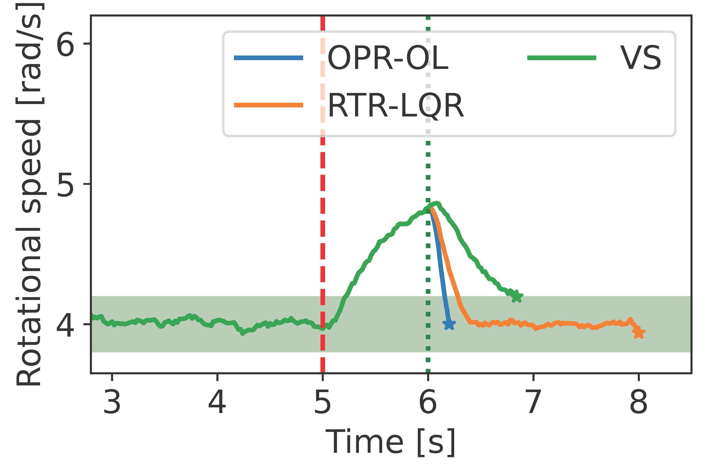
We present the simulations for the Fast Attack Recovery for Stochastic Cyber-Physical Systems paper [4]. We propose the solution to the Optimal probabilistic recovery (OPR). We use the linear model of a motor as an example. For the experiments in the paper, we simulate a bias attack against the motor angular speed measurement by adding a bias of -1m/s. The adversary deploys the attack at time 3s after beginning the simulation, and the detector identifies the attack one second later. This alarm triggers the recovery strategies.

We compare the performance of our solution, called the open loop OPR (OPR-OL), with the LQR-based recovery [2]_, and virtual sensors. We then obtain the next Figure:

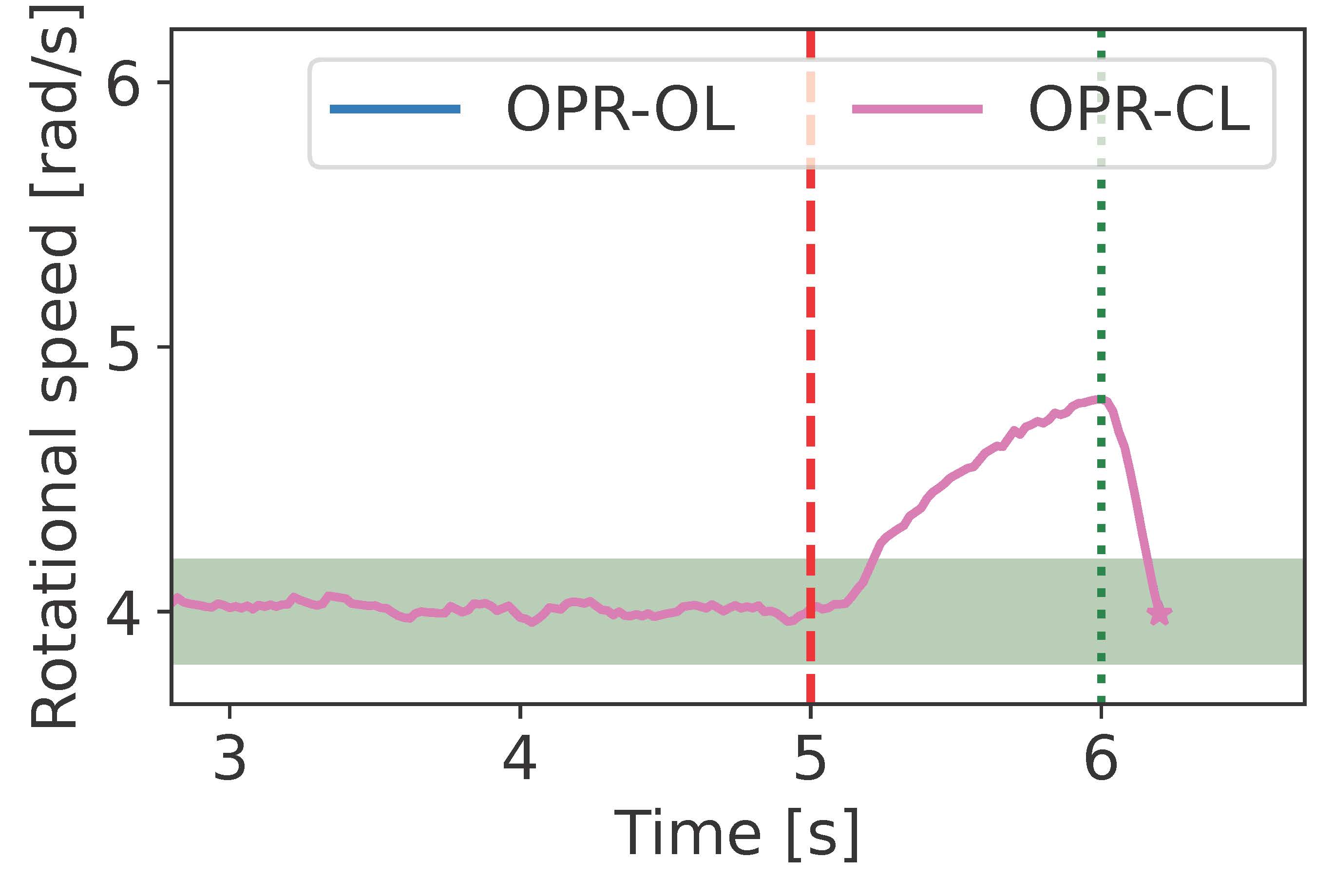
We also include the simulations to improve our solution by incorporating the non-compromised sensors into the recovery. We call this strategy the partially closed loop OPR (OPR-PCL). We compare the OPR-OL and OPR-PCL:

We provide the code to obtain previous figures.

Bias attack on the CSTR benchmark

'''
This file implements the simulation of real-time recovery linear quadratic regulator (RTR-LQR)
Virtual sensors (VS), Optimal probabilistic recovery in open loop (OPR-OL) and closed loop (OPR-CL)
'''

from copy import deepcopy
import matplotlib.pyplot as plt
plt.rcParams.update({'font.size': 15})
import matplotlib
matplotlib.rcParams['pdf.fonttype'] = 42
matplotlib.rcParams['ps.fonttype'] = 42

import numpy as np
import logging
import sys
import os
import csv
import time
from time import perf_counter

os.environ["RANDOM_SEED"] = '0'   # for reproducibility
sys.path.append(sys.path[0] + '/../../')

from cpsim.formal.gaussian_distribution import GaussianDistribution
from cpsim.formal.reachability import ReachableSet
from cpsim.formal.zonotope import Zonotope
from cpsim.observers.kalman_filter import KalmanFilter
from cpsim.observers.full_state_bound import Estimator
from cpsim.controllers.LP_cvxpy import LP
from cpsim.controllers.MPC_cvxpy import MPC

# from cpsim.performance.performance_metrics import distance_to_strip_center, in_strip

def in_strip(l, x, a, b):
    if l @ x >= a and l @ x <= b:
        success = 1
    else:
        success = 0
    return success

colors = {'none': 'red', 'lqr': 'C1', 'ssr': 'C2', 'oprp-close': 'C4', 'oprp-open': 'C0'}
labels = {'none': 'None', 'lqr': 'RTR-LQR', 'ssr': 'VS', 'oprp-close': 'OPR-PCL', 'oprp-open': 'OPR'}

# logger
logging.basicConfig(
    format="%(asctime)s [%(levelname)s] %(message)s",
    handlers=[
        logging.FileHandler("debug.log"),
        logging.StreamHandler(sys.stdout)
    ]
)
logger = logging.getLogger(__name__)
logger.setLevel(logging.DEBUG)






def save_exp_data(exp, exp_rst, bl, profiling_data = None):
    '''method to store data'''
    exp_rst[bl]['states'] = deepcopy(exp.model.states)
    exp_rst[bl]['outputs'] = deepcopy(exp.model.outputs)
    exp_rst[bl]['inputs'] = deepcopy(exp.model.inputs)
    exp_rst[bl]['time'] = {}

    exp_rst[bl]['recovery_steps'] = profiling_data['recovery_steps']
    exp_rst[bl]['recovery_complete_index'] = profiling_data['recovery_complete_index']
    
        

# ---------  attack + no recovery  -------------
def simulate_no_recovery(exp, bl):
    '''
    Simulation with attack and no recovery
    exp: class with the experiment characteristics
    '''
    exp.model.reset()
    exp_name = f" {bl} {exp.name} "
    logger.info(f"{exp_name:=^40}")
    for i in range(0, exp.max_index + 1):
        assert exp.model.cur_index == i
        exp.model.update_current_ref(exp.ref[i])
        # attack here
        exp.model.cur_feedback = exp.attack.launch(exp.model.cur_feedback, i, exp.model.states)
        exp.model.evolve()

    profiling_data = {}
    profiling_data["recovery_complete_index"] = exp.max_index + 1
    profiling_data["recovery_steps"] = exp.max_index - exp.attack_start_index 
    
    return profiling_data


# ---------  LQR  -------------
def simulate_LQR(exp, bl):
    '''
    Simulate the RTR-LQR
    '''
    exp_name = f" {bl} {exp.name} "
    logger.info(f"{exp_name:=^40}")
    # required objects
    A = exp.model.sysd.A
    B = exp.model.sysd.B
    est = Estimator(A, B, max_k=150, epsilon=1e-7)
    maintain_time = 3
    exp.model.reset()
    # init variables
    recovery_complete_index = exp.max_index
    rec_u = None

    elapsed_times = []
    # Main loop 
    for i in range(0, exp.max_index + 1):
        assert exp.model.cur_index == i
        # Obtains reference
        exp.model.update_current_ref(exp.ref[i])
        # Launch attack
        exp.model.cur_feedback = exp.attack.launch(exp.model.cur_feedback, i, exp.model.states)
        if i == exp.attack_start_index - 1:
            logger.debug(f'trustworthy_index={i}, trustworthy_state={exp.model.cur_x}')
            pass

        
        # Check if the recovery begins
        if i == exp.recovery_index:
            logger.debug(f'recovery_index={i}, recovery_start_state={exp.model.cur_x}')

            # State reconstruction
            us = exp.model.inputs[exp.attack_start_index - 1:exp.recovery_index]
            x_0 = exp.model.states[exp.attack_start_index - 1]
            x_cur_lo, x_cur_up, x_cur = est.estimate(x_0, us)
            logger.debug(f'reconstructed state={x_cur}')

            # deadline estimate
            safe_set_lo = exp.safe_set_lo
            safe_set_up = exp.safe_set_up
            control = exp.model.inputs[i - 1]
            k = est.get_deadline(x_cur, safe_set_lo, safe_set_up, control, 100)
            recovery_complete_index = exp.recovery_index + k
            logger.debug(f'deadline={k}')
            # maintainable time compute


            # get recovery control sequence
            lqr_settings = {
                'Ad': A, 'Bd': B,
                'Q': exp.Q, 'QN': exp.QN, 'R': exp.R,
                'N': k + 3,
                'ddl': k, 'target_lo': exp.target_set_lo, 'target_up': exp.target_set_up,
                'safe_lo': exp.safe_set_lo, 'safe_up': exp.safe_set_up,
                'control_lo': exp.control_lo, 'control_up': exp.control_up,
                'ref': exp.recovery_ref
            }
            lqr = MPC(lqr_settings)
            _ = lqr.update(feedback_value=x_cur)
            rec_u = lqr.get_full_ctrl()
            rec_x = lqr.get_last_x()
            logger.debug(f'expected recovery state={rec_x}')
        # Implements the RTR-LQR recovery
        if i == recovery_complete_index + maintain_time:
            logger.debug(f'state after recovery={exp.model.cur_x}')
            step = recovery_complete_index + maintain_time - exp.recovery_index
            logger.debug(f'use {step} steps to recover.')
        # Check we need to use the recovery
        if exp.recovery_index <= i < recovery_complete_index + maintain_time:
            rec_u_index = i - exp.recovery_index
            u = rec_u[rec_u_index]
            exp.model.evolve(u)
        else: # If not using the recovery, run one step
            exp.model.evolve()
    # Store profiling data
    profiling_data = {}
    profiling_data["recovery_complete_index"] = recovery_complete_index
    profiling_data["recovery_steps"] = step
    return profiling_data


# ---------  attack + virtual sensors  -------------
def simulate_ssr(exp, bl):
    '''
    Implements the software sensors
    '''
    # required objects
    recovery_complete_index = exp.max_index - 1
    A = exp.model.sysd.A
    B = exp.model.sysd.B
    est = Estimator(A, B, max_k=150, epsilon=1e-7)
    logger.info(f"{bl} {exp.name:=^40}")
    for i in range(0, exp.max_index + 1):
        assert exp.model.cur_index == i
        exp.model.update_current_ref(exp.ref[i])
        # attack here
        exp.model.cur_feedback = exp.attack.launch(exp.model.cur_feedback, i, exp.model.states)

        if i == exp.attack_start_index - 1:
            logger.debug(f'trustworthy_index={i}, trustworthy_state={exp.model.cur_x}')
            pass
        if i == exp.recovery_index:
            logger.debug(f'recovery_index={i}, recovery_start_state={exp.model.cur_x}')

            # State reconstruction
            us = exp.model.inputs[exp.attack_start_index - 1:exp.recovery_index]
            x_0 = exp.model.states[exp.attack_start_index - 1]
            x_cur = est.estimate_wo_bound(x_0, us)
            logger.debug(f'one before reconstructed state={x_cur}')
            last_predicted_state = deepcopy(x_cur)

        if exp.recovery_index <= i < recovery_complete_index:
            # check if it is in target set
            if in_strip(exp.s.l, last_predicted_state, exp.s.a, exp.s.b):
                recovery_complete_index = i
                logger.debug('state after recovery={exp.model.cur_x}')
                step = recovery_complete_index - exp.recovery_index
                logger.debug(f'use {step} steps to recover.')
            
            # Estimate the state using the virtual sensors
            us = [exp.model.inputs[i - 1]]
            x_0 = last_predicted_state
            x_cur = est.estimate_wo_bound(x_0, us)

            # Set the feedback to the state estimated by the virtual sensors
            exp.model.cur_feedback = exp.model.sysd.C @ x_cur
            last_predicted_state = deepcopy(x_cur)
            print(f'{exp.model.cur_u}')


        exp.model.evolve()
    
    profiling_data = {}
    profiling_data["recovery_complete_index"] = recovery_complete_index
    profiling_data["recovery_steps"] = recovery_complete_index - exp.recovery_index 
    return profiling_data


# ---------  attack + OPR-CL  -------------
def simulate_oprp_cl(exp, bl):
    '''
    Simulate the OPR-CL
    exp: class with the experiments characteristics.
    '''
    # required objects
    A = exp.model.sysd.A
    B = exp.model.sysd.B
    # Initialize the Kalman filter
    kf_C = exp.kf_C
    C = exp.model.sysd.C
    D = exp.model.sysd.D
    kf_Q = exp.model.p_noise_dist.sigma if exp.model.p_noise_dist is not None else np.zeros_like(A)
    kf_R = exp.kf_R
    kf = KalmanFilter(A, B, kf_C, D, kf_Q, kf_R)
    # Initialize the zonotopes
    U = Zonotope.from_box(exp.control_lo, exp.control_up)
    W = exp.model.p_noise_dist
    reach = ReachableSet(A, B, U, W, max_step=exp.max_recovery_step )

    # init variables
    recovery_complete_index = exp.max_index
    x_cur_update = None

    
    
    logger.info(f" OPR-CL {exp.name} ")
    for i in range(0, exp.max_index + 1):
        assert exp.model.cur_index == i
        exp.model.update_current_ref(exp.ref[i])
        # attack here
        exp.model.cur_feedback = exp.attack.launch(exp.model.cur_feedback, i, exp.model.states)

        if i == exp.attack_start_index - 1:
            logger.debug(f'trustworthy_index={i}, trustworthy_state={exp.model.cur_x}')
            pass

        # state reconstruct
        if i == exp.recovery_index:
            logger.debug(f'recovery_index={i}, recovery_start_state={exp.model.cur_x}')
            # Obtains the inputs between instant of the attack beginning and the recovery beginning
            us = exp.model.inputs[exp.attack_start_index-1:exp.recovery_index]
            # Obtains the measurements.
            ys = (kf_C @ exp.model.states[exp.attack_start_index:exp.recovery_index + 1].T).T
            x_0 = exp.model.states[exp.attack_start_index-1]
            # Use a Kalman filter to estimate the state at the reconfiguration beginning
            x_res, P_res = kf.multi_steps(x_0, np.zeros_like(A), us, ys)
            x_cur_update = GaussianDistribution(x_res[-1], P_res[-1])
            logger.debug(f"reconstructed state={x_cur_update.miu=}, ground_truth={exp.model.cur_x}")
        # OPR-OL recovery begins
        # Estimate the probability distribution of the system state
        if exp.recovery_index < i < recovery_complete_index:
            x_cur_predict = GaussianDistribution(*kf.predict(x_cur_update.miu, x_cur_update.sigma, exp.model.cur_u))
            y = kf_C @ exp.model.cur_x
            x_cur_update = GaussianDistribution(*kf.update(x_cur_predict.miu, x_cur_predict.sigma, y))
            logger.debug(f"reconstructed state={x_cur_update.miu=}, ground_truth={exp.model.cur_x}")

        if i == recovery_complete_index:
            logger.debug(f'state after recovery={exp.model.cur_x}')
            pass
        # Use the OPR-OL to implement the recovery
        if exp.recovery_index <= i < recovery_complete_index:
            # Compute the reachable means
            reach.init(x_cur_update, exp.s)
            # Compute the recovery sequence
            k, X_k, D_k, z_star, alpha, P, arrive = reach.given_k(max_k=exp.max_recovery_step)
            print(f"{k=}, {z_star=}, {P=}")
            recovery_control_sequence = U.alpha_to_control(alpha)
            recovery_complete_index = i+k
            exp.model.evolve(recovery_control_sequence[0])
            print(f"{i=}, {recovery_control_sequence[0]=}")
        else:
            exp.model.evolve()
    
    profiling_data = {}
    profiling_data["recovery_complete_index"] = recovery_complete_index
    profiling_data["recovery_steps"] = recovery_complete_index - exp.recovery_index 
    return profiling_data

# ---------  attack + OPR_OL  -------------
def simulate_oprp_ol(exp, bl):
    '''
    function to simulate the OPR-OL strategy.
    exp: the experiment settings class 
    '''
    # required objects
    A = exp.model.sysd.A
    B = exp.model.sysd.B
    C = exp.model.sysd.C
    U = Zonotope.from_box(exp.control_lo, exp.control_up)
    W = exp.model.p_noise_dist
    reach = ReachableSet(A, B, U, W, max_step=exp.max_recovery_step )

    # init variables
    recovery_complete_index = exp.max_index
    x_cur_update = None
    exp_name = f" OPR-OL {exp.name} "
    logger.info(f"{exp_name:=^40}")
    for i in range(0, exp.max_index + 1):
        assert exp.model.cur_index == i
        exp.model.update_current_ref(exp.ref[i])
        # attack here
        exp.model.cur_feedback = exp.attack.launch(exp.model.cur_feedback, i, exp.model.states)
        if i == exp.attack_start_index - 1:
            logger.debug(f'trustworthy_index={i}, trustworthy_state={exp.model.cur_x}')
            pass

        # state reconstruct
        if i == exp.recovery_index:
            us = exp.model.inputs[exp.attack_start_index - 1:exp.recovery_index]
            x_0 = exp.model.states[exp.attack_start_index - 1]
            x_0 = GaussianDistribution(x_0, np.zeros((exp.model.n, exp.model.n)))
            reach.init(x_0, exp.s)
            x_res_point = reach.state_reconstruction(us)
            print('x_0=', x_res_point)

            reach.init(x_res_point, exp.s)
            k, X_k, D_k, z_star, alpha, P, arrive = reach.given_k(max_k=exp.k_given)
            recovery_complete_index = exp.recovery_index + k
            rec_u = U.alpha_to_control(alpha)
            
            print('k=', k, 'P=', P, 'z_star=', z_star, 'arrive=', arrive)
            print('D_k=', D_k)
            print('recovery_complete_index=', recovery_complete_index)
            print(rec_u)

        if exp.recovery_index <= i < recovery_complete_index:
            rec_u_index = i - exp.recovery_index
            u = rec_u[rec_u_index]
            exp.model.evolve(u)
        else:
            exp.model.evolve()
    
    profiling_data = {}
    profiling_data["recovery_complete_index"] = recovery_complete_index
    profiling_data["recovery_steps"] = recovery_complete_index - exp.recovery_index 

    return profiling_data

def plot_ts(strategies, exp, exp_rst):
    plt.figure(figsize=(5,3))
    max_t = 0
    for strategy in strategies:
        # 
        states = exp_rst[strategy]["states"]
        t = np.arange(0, len(states)) * exp.dt

        states = states[0:exp_rst[strategy]["recovery_complete_index"] + 1]
        t = t[0:exp_rst[strategy]["recovery_complete_index"] + 1]
        max_t = np.maximum(t[-1], max_t)
        #
        plt.plot(t, states[:, 0], color=colors[strategy], label=labels[strategy], linewidth=2)
        plt.plot(t[-1], states[-1, 0], color=colors[strategy], marker='*', linewidth=8)
    # Plot limits in x
    axes = plt.gca()
    x_lim = axes.get_xlim()
    plt.xlim(exp.x_lim[0], max_t + 0.5)

    # Plot limits in y
    plt.ylim(exp.y_lim)
    plt.vlines(exp.attack_start_index * exp.dt, exp.y_lim[0], exp.y_lim[1], color='red', linestyle='dashed', linewidth=2)
    plt.vlines(exp.recovery_index * exp.dt, exp.y_lim[0], exp.y_lim[1], colors='green', linestyle='dotted', linewidth=2)

    plt.fill_between(t + 0.5, t * 0 - exp.s.a, t * 0 - exp.s.b, facecolor='green', alpha=0.3)
    plt.ylabel(exp.y_label)
    plt.xlabel("Time [s]")
    plt.legend(ncol=2)


def sim_strategies(exps, plot_time_series):
    
    for exp in exps:

        strategies = {}
        # Declare strategies we want to simulate
        strategies = {  # 'none': simulate_no_recovery,
                        'ssr': simulate_ssr,
                        'oprp-close': simulate_oprp_cl,
                        'oprp-open': simulate_oprp_ol,
                        'lqr': simulate_LQR}
        
        
        result = {}
        result[exp.name] = {}
        exp_rst = result[exp.name]
        for strategy in strategies:
            exp.model.reset()
            exp_rst[strategy] = {}
            simulate = strategies[strategy]
            # Simulate strategy
            profiling_data = simulate(exp, strategy)
            # Store data
            save_exp_data(exp, exp_rst, strategy, profiling_data)
            recovery_complete_index = exp_rst[strategy]['recovery_complete_index']
            final_state = exp_rst[strategy]['states'][recovery_complete_index].tolist()
            

            
        # Begin plots 
        if plot_time_series:
            str_plot = ['ssr', 'oprp-open', 'lqr']
            plot_ts(str_plot, exp, exp_rst)
            str_plot = ['oprp-open', 'oprp-close']
            plot_ts(str_plot, exp, exp_rst)
            plt.show()
            


# Main function
def main():
    plot_time_series = True
    # Import the system and simulation settings. See the settings.py file
    # This classes have the simulation parameters such as the safe regions
    from settings import motor_speed_bias, quadruple_tank_bias, f16_bias, aircraft_pitch_bias, boeing747_bias, quadrotor_bias, rlc_circuit_bias
    exps = [motor_speed_bias]
    sim_strategies(exps, plot_time_series)

    
if __name__ == "__main__":
    main()
    
        

An user can change the attack characteristics (e.g., detection delay).

Bias attack on the CSTR benchmark

'''
This file has the simulation parameters for several linear systems presented in the paper.
'''

import numpy as np
import sys
sys.path.append(sys.path[0] + '/../')
from cpsim.models.linear.motor_speed import MotorSpeed
from cpsim.models.linear.quadruple_tank import QuadrupleTank
from cpsim.models.linear.F16 import F16
from cpsim.models.linear.aircraft_pitch import AircraftPitch
from cpsim.models.linear.boeing747 import Boeing
from cpsim.models.linear.heat import Heat
from cpsim.models.linear.platoon import Platoon
from cpsim.models.linear.rlc_circuit import RlcCircuit
from cpsim.models.linear.quadrotor import Quadrotor
from cpsim.models.linear.lane_keeping import LaneKeeping
from cpsim.attack import Attack
from cpsim.formal.strip import Strip
# --------------------- motor speed -------------------
class motor_speed_bias:
    # Experiment name
    name = 'motor_speed_bias'
    # Maximum simulation steps
    max_index = 500
    # Discretization time
    dt = 0.02
    # Reference vector
    ref = [np.array([4])] * 501
    # Noise characteristics
    noise = {
        'process': {
            'type': 'white',
            'param': {'C': np.array([[0.01, 0], [0, 0.01]])}
        }
    }
    # Import system dynamics
    model = MotorSpeed('bias', dt, max_index, noise)
    # Control input constraints
    control_lo = np.array([0])
    control_up = np.array([50])
    model.controller.set_control_limit(control_lo, control_up)
    # Attack characteristics
    attack_start_index = 150
    bias = np.array([-1])
    attack = Attack('bias', bias, attack_start_index)
    # Attacks detection instant. This value comes from the detector.
    recovery_index = 200

    # OPR parameters: strip vector l and parameters a, b
    s = Strip(np.array([-1, 0]), a=-4.2, b=-3.8)
    P_given = 0.95
    max_recovery_step = 140
    # plot
    ref_index = 0

    # Kalman filter parameters for the OPR-CL
    kf_C = np.array([[0, 1]]) # This parameter depends on the attack characteristics
    k_given = 40   # This is K. Maximum number of recovery steps
    kf_R = np.diag([1e-7])

    # Parameters for the RTR-LQR 
    safe_set_lo = np.array([4, 30])
    safe_set_up = np.array([5.07, 80])
    target_set_lo = np.array([3.8, 35.81277766])
    target_set_up = np.array([4.2, 60])
    recovery_ref = np.array([4,  41.81277766])
    Q = np.diag([100, 1])
    QN = np.diag([100, 1])
    R = np.diag([1])
    
    # Plot 
    output_index = 0
    x_lim = (2.8, 4.2)
    y_lim = (3.65, 5.2)
    y_label = 'Rotational speed [rad/s]'
    strip = (4.2, 3.8)


# -------------------- quadruple tank ----------------------------
class quadruple_tank_bias:
    # Experiment name
    name = 'quadruple_tank_bias'
    # Maximum simulation steps
    max_index = 300
    # Discretization time
    dt = 1
    # Reference vector
    ref = [np.array([7, 7])] * 1001 + [np.array([7, 7])] * 1000
    # Noise characteristics
    noise = {
        'process': {
            'type': 'white',
            'param': {'C': np.diag([0.05, 0.05, 0.05, 0.05])}
        }
    }
    # Import system dynamics
    model = QuadrupleTank('test', dt, max_index, noise)
    # Control input constraints
    control_lo = np.array([0, 0])
    control_up = np.array([10, 10])
    model.controller.set_control_limit(control_lo, control_up)
    # Attack characteristics
    attack_start_index = 150
    bias = np.array([-2.0, 0])
    attack = Attack('bias', bias, attack_start_index)
    recovery_index = 160


    # OPR parameters: strip vector l and parameters a, b
    s = Strip(np.array([-1, 0, 0, 0]), a=-14.3, b=-13.7)
    P_given = 0.95
    max_recovery_step = 140

    # Kalman filter parameters for the OPR-CL
    kf_C = np.array([[0, 1, 0, 0], [0, 0, 1, 0], [0, 0, 0, 1]])  # depend on attack
    k_given = 40 # This is K. Maximum number of recovery steps
    kf_R = np.diag([1e-7, 1e-7, 1e-7])

    # Parameters for the RTR-LQR 
    safe_set_lo = np.array([0, 0, 0, 0])
    safe_set_up = np.array([20, 20, 20, 20])
    target_set_lo = np.array([13.8, 13.8, 0, 0])
    target_set_up = np.array([14.2, 14.2, 20, 20])
    recovery_ref = np.array([14, 14, 2, 2.5])
    Q = np.diag([1, 1, 0, 0])
    QN = np.diag([1, 1, 0, 0])
    R = np.diag([1, 1])
    

    # plot
    ref_index = 0
    output_index = 0
    x_lim = (140, 200)
    y_lim = (6.7, 9)
    y_label = 'water level - cm'
    strip = (7.15, 6.85)  # modify according to strip


# -------------------- f16 ----------------------------
class f16_bias:
    # Experiment name
    name = 'f16_bias'
    # Maximum simulation steps
    max_index = 550
    # Discretization time
    dt = 0.02
    # Reference vector
    ref = [np.array([0.0872665 * 57.3])] * 801
    # Noise characteristics
    noise = {
        'process': {
            'type': 'white',
            'param': {'C': np.eye(4) * 0.002}
        }
    }
    # Import system dynamics
    model = F16('test', dt, max_index, noise)
    # Control input constraints
    control_lo = np.array([-25])
    control_up = np.array([25])
    model.controller.set_control_limit(control_lo, control_up)
    # Attack characteristics
    attack_start_index = 400
    bias = np.array([-10])
    attack = Attack('bias', bias, attack_start_index)
    recovery_index = 470


    # OPR parameters: strip vector l and parameters a, b
    s = Strip(np.array([0, 0, 1, 0]), a=4.2/57.3, b=5.8/57.3)
    P_given = 0.95
    max_recovery_step = 140

    # Kalman filter parameters for the OPR-CL
    kf_C = np.array([[1, 0, 0, 0], [0, 1, 0, 0], [0, 0, 0, 1]])  # depend on attack
    k_given = 40 # This is K. Maximum number of recovery steps
    kf_R = np.diag([1e-7, 1e-7, 1e-7])
    

    # Parameters for the RTR-LQR 
    safe_set_lo = np.array([300, -5.01717652e-01, 0.04, -1])
    safe_set_up = np.array([5.02135552e+02,1.01717652e-01, 0.116, 1])
    target_set_lo = np.array([3.52135331e+02, -1.51738001e-01,  0.0871,  3.05954232e-04])
    target_set_up = np.array([4.52135331e+02,  -0.51738001e-01, 0.0873,  4.05954232e-04])
    recovery_ref = np.array([4.02135552e+02, -1.01717652e-01, 0.0872665, 1.83150103e-04])
    Q = np.diag([1, 1, 10000, 10000])
    QN = np.diag([1, 1, 10000, 10000])
    R = np.diag([1])

    # Plots 
    ref_index = 0
    output_index = 0
    x_lim = (7.9, 8.95)
    y_lim = (4.5, 6.7)
    y_label = 'pitch angle - degree'
    strip = (5.1, 4.9)
    


# -------------------- aircraft_pitch ----------------------------
class aircraft_pitch_bias:
    # Experiment name
    name = 'aircraft_pitch_bias'
    # Maximum simulation steps
    max_index = 1500
    # Discretization time
    dt = 0.02
    # Reference vector
    ref = [np.array([0.2])] * (max_index + 1)
    # Noise characteristics
    noise = {
        'process': {
            'type': 'white',
            'param': {'C': np.diag([0.0003, 0.0002, 0.0003])}
        }
    }
    # Import system dynamics
    model = AircraftPitch('aircraft_pitch', dt, max_index, noise)
    # Control input constraints
    control_lo = np.array([-20])
    control_up = np.array([20])
    model.controller.set_control_limit(control_lo, control_up)
    # Attack characteristics
    attack_start_index = 500
    bias = np.array([-1])
    attack = Attack('bias', bias, attack_start_index)
    recovery_index = 550


    # OPR parameters: strip vector l and parameters a, b
    s = Strip(np.array([0, 0, -1]), a=-0.395, b=-0.005)
    P_given = 0.95
    max_recovery_step = 140

    # Kalman filter parameters for the OPR-CL
    kf_C = np.array([[1, 0, 0], [0, 1, 0]])  # depend on attack
    k_given = 40 # This is K. Maximum number of recovery steps
    kf_R = np.diag([1e-7, 1e-7])

    # baseline
    safe_set_lo = np.array([-5,    -5, 0])
    safe_set_up = np.array([5,    5, 1.175])
    target_set_lo = np.array([0.01624,    0.0, 0.19])
    target_set_up = np.array([0.05624,  0.01, 0.21])
    recovery_ref = np.array([0.05624,    0.00028221, 0.2])
    Q = np.diag([1, 100000, 100000])
    QN = np.diag([1, 100000, 100000])
    R = np.diag([1])

    # plot
    ref_index = 0
    output_index = 0
    x_lim = (9.7, 12.7)
    y_lim = (0, 1.3)
    y_label = 'pitch - rad'
    strip = (0.23, 0.17)


# -------------------- boeing747 ----------------------------
class boeing747_bias:
    # Experiment name
    name = 'boeing747'
    # Maximum simulation steps
    max_index = 800
    # Discretization time
    dt = 0.02
    # Reference vector
    ref = [np.array([1])] * (max_index + 1)
    # Noise characteristics
    noise = {
        'process': {
            'type': 'white',
            'param': {'C': np.eye(5) * 0.02}
        }
    }
    # Import system dynamics
    model = Boeing('boeing747', dt, max_index, noise)
    # Control input constraints
    control_lo = np.array([-30])
    control_up = np.array([30])
    model.controller.set_control_limit(control_lo, control_up)
    # Attack characteristics
    attack_start_index = 400
    bias = np.array([-1])
    attack = Attack('bias', bias, attack_start_index)
    recovery_index = 430


    # OPR parameters: strip vector l and parameters a, b
    s = Strip(np.array([-1, 0, 0, 0, 0]), a=-1.4, b=-0.6)
    P_given = 0.95
    max_recovery_step = 140

    # Kalman filter parameters for the OPR-CL
    kf_C = np.array([[0, 1, 0, 0, 0], [0, 0, 1, 0, 0], [0, 0, 0, 1, 0], [0, 0, 0, 0, 1]])  # depend on attack
    k_given = 40 # This is K. Maximum number of recovery steps
    kf_R = np.diag([1e-7, 1e-7, 1e-7, 1e-7])

    # baseline
    safe_set_lo = np.array([0.0, -10, -5, -5, -30])
    #safe_set_up = np.array([1.817344443758, 5, 5, 50, 15])
    safe_set_up = np.array([1.819, 5, 20, 50, 25])
    target_set_lo = np.array([0.9, -10, -10, -10, -100])
    target_set_up = np.array([1.1, 10, 100, 100, 100])
    recovery_ref = np.array([1, 0, 0, 0, 0])
    Q = np.diag([100000, 1, 10000, 1, 1])
    QN = np.diag([100000, 1, 10000, 1, 1])
    R = np.diag([1]) * 0.1

    # plot
    ref_index = 0
    output_index = 0
    x_lim = (7.8,9.5)
    y_lim = (0.7, 2.0)
    y_label = 'Yaw angle - rad'
    strip = (0.85, 1.15)

def generate_list(dimension, value):
    temp = []
    for i in range(dimension):
        temp.append(value)
    return temp
# -------------------- heat ----------------------------
class heat_bias:
    # Experiment name
    name = 'heat'
    # Maximum simulation steps
    max_index = 1000
    # Discretization time
    dt = 1
    # Reference vector
    ref = [np.array([15])] * (max_index + 1)
    # Noise characteristics
    noise = {
        'process': {
            'type': 'white',
            'param': {'C': np.eye(45) * 0.0001}
        }
    }
    # Import system dynamics
    model = Heat('heat', dt, max_index, noise)
    # Control input constraints
    control_lo = np.array([-0.5])
    control_up = np.array([50])
    model.controller.set_control_limit(control_lo, control_up)
    # Attack characteristics
    attack_start_index = 400
    bias = np.array([-1])
    attack = Attack('bias', bias, attack_start_index)
    recovery_index = 500


    l = np.zeros((45,))
    y_point = (45 + 1) // 3 * 2 - 1
    l[y_point] = -1
    # OPR parameters: strip vector l and parameters a, b
    s = Strip(l, a=-15.3, b=-14.7)
    P_given = 0.95
    max_recovery_step = 160
    # plot
    ref_index = 0
    output_index = 0

    kf_C = np.zeros((44, 45))  # depend on attack
    for i in range(44):
        if i < y_point:
            kf_C[i][i] = 1
        elif i >= y_point:
            kf_C[i][i + 1] = 1
    k_given = 40 # This is K. Maximum number of recovery steps
    temp = []
    for i in range(44):
        temp.append(1e-7)
    kf_R = np.diag(temp)

    # baseline
    temp = generate_list(45, -10)
    safe_set_lo = np.array(temp)

    temp = generate_list(45, 1000)
    safe_set_up = np.array(temp)

    temp = generate_list(45, -10)
    temp[y_point] = 14.8
    target_set_lo = np.array(temp)

    temp = generate_list(45, 1000)
    temp[y_point] = 15.2
    target_set_up = np.array(temp)

    temp = generate_list(45, 0)
    temp[y_point] = 15
    recovery_ref = np.array(temp)

    temp = generate_list(45, 1)
    temp[y_point] = 1
    Q = np.diag(temp)
    QN = np.diag(temp)
    R = np.diag([1]) * 10000





# -------------------- platoon ----------------------------
class platoon_bias:
    # Experiment name
    name = 'platoon'
    # Maximum simulation steps
    max_index = 800
    # Discretization time
    dt = 0.02
    # Reference vector
    ref = [np.array([2])] * (max_index + 1)
    # Noise characteristics
    noise = {
        'process': {
            'type': 'white',
            'param': {'C': np.eye(7) * 0.0001}
        }
    }
    # Import system dynamics
    model = Platoon('Platoon', dt, max_index, noise)
    # Control input constraints
    control_lo = np.array([-5, -5, -5, -5])
    control_up = np.array([5, 5, 5, 5])
    model.controller.set_control_limit(control_lo, control_up)
    # Attack characteristics
    attack_start_index = 400
    bias = np.array([-1])
    attack = Attack('bias', bias, attack_start_index)
    recovery_index = 450


    # OPR parameters: strip vector l and parameters a, b
    s = Strip(np.array([-1, 0, 0, 0, 0, 0, 0]), a=-2.3, b=-1.7)
    P_given = 0.95
    max_recovery_step = 140
    # plot
    ref_index = 0
    output_index = 0
    x_lim = (7.5,10)
    y_lim = (1.5, 2.7)
    y_label = 'relative distance error with car 1 and 2'
    strip = (1.9, 2.1)

    kf_C = np.array([[0, 1, 0, 0, 0, 0, 0], [0, 0, 1, 0, 0, 0, 0], [0, 0, 0, 1, 0, 0, 0],
                     [0, 0, 0, 0, 1, 0, 0], [0, 0, 0, 0, 0, 1, 0], [0, 0, 0, 0, 0, 0, 1]])  # depend on attack
    k_given = 40 # This is K. Maximum number of recovery steps
    kf_R = np.diag([1e-7, 1e-7, 1e-7, 1e-7, 1e-7, 1e-7])

    # baseline
    safe_set_lo = np.array([1, 1, 1, 0, 0, 0, 0])
    safe_set_up = np.array([2.5, 3, 3, 5, 5, 5, 5])
    target_set_lo = np.array([1.95, 0, 0, 0, 0, 0, 0])
    target_set_up = np.array([2.05, 5, 5, 5, 5, 5, 5])
    recovery_ref = np.array([2, 2, 2, 2, 2, 2, 2])
    Q = np.diag([1, 1, 1, 1, 1, 1, 1])
    QN = np.diag([1, 1, 1, 1, 1, 1, 1])
    R = np.diag([1, 1, 1, 1])


# -------------------- rlc_circuit ----------------------------
class rlc_circuit_bias:
    # Experiment name
    name = 'rlc_circuit'
    # Maximum simulation steps
    max_index = 800
    # Discretization time
    dt = 0.02
    # Reference vector
    ref = [np.array([3])] * (max_index + 1)
    # Noise characteristics
    noise = {
        'process': {
            'type': 'white',
            'param': {'C': np.eye(2) * 0.0001}
        }
    }
    # Import system dynamics
    model = RlcCircuit('rlc_circuit', dt, max_index, noise)
    # Control input constraints
    control_lo = np.array([-15])
    control_up = np.array([15])
    model.controller.set_control_limit(control_lo, control_up)
    # Attack characteristics
    attack_start_index = 400
    bias = np.array([-1])
    attack = Attack('bias', bias, attack_start_index)
    recovery_index = 415


    # OPR parameters: strip vector l and parameters a, b
    s = Strip(np.array([-1, 0]), a=-3.2, b=-2.8)
    P_given = 0.95
    max_recovery_step = 140
    # plot
    ref_index = 0
    output_index = 0
    x_lim = (7.9, 8.7)
    y_lim = (2.7, 4.1)
    y_label = 'Capacitor Voltage - V'
    strip = (2.8, 3.2)

    kf_C = np.array([[0, 1]])  # depend on attack
    k_given = 40 # This is K. Maximum number of recovery steps
    kf_R = np.diag([1e-7])

    # baseline
    safe_set_lo = np.array([2.5, -1])
    safe_set_up = np.array([4, 0.5])
    target_set_lo = np.array([2.95, -1])
    target_set_up = np.array([3.05, 1])
    recovery_ref = np.array([3, -1.52863266e-05])
    Q = np.diag([1, 1])
    QN = np.diag([1, 1])
    R = np.diag([1])


# -------------------- quadrotor ----------------------------
class quadrotor_bias:
    # Experiment name
    name = 'quadrotor'
    # Maximum simulation steps
    max_index = 1000
    # Discretization time
    dt = 0.02
    # Reference vector
    ref = [np.array([4])] * (max_index + 1)
    # Noise characteristics
    noise = {
        'process': {
            'type': 'white',
            'param': {'C': np.eye(12) * 0.08}
        }
    }
    # Import system dynamics
    model = Quadrotor('quadrotor', dt, max_index, noise)
    # Control input constraints
    control_lo = np.array([-50])
    control_up = np.array([50])
    model.controller.set_control_limit(control_lo, control_up)
    # Attack characteristics
    attack_start_index = 400
    bias = np.array([-2])
    attack = Attack('bias', bias, attack_start_index)
    recovery_index = 410


    # OPR parameters: strip vector l and parameters a, b
    s = Strip(np.array([0, 0, 0, 0, 0, 0, 0, 0, 0, 0, 0, -1]), a=-4.5, b=-3.5)
    P_given = 0.95
    max_recovery_step = 140
    # plot
    ref_index = 0
    output_index = 5
    x_lim = (7.9, 8.9)
    y_lim = (3.5, 6.2)
    y_label = 'Altitude - m'
    strip = (4.3, 3.7)

    # kf_C = np.array([[0, 0, 0, 0, 0, 0, 0, 0, 0, 0, 0, 0]])  # depend on attack
    kf_C = np.zeros((11, 12))
    for i in range(11):
        kf_C[i][i] = 1
    # print(kf_C)
    k_given = 40 # This is K. Maximum number of recovery steps
    kf_R = np.diag([1e-7, 1e-7, 1e-7, 1e-7, 1e-7, 1e-7, 1e-7, 1e-7, 1e-7, 1e-7, 1e-7])

    # baseline
    safe_set_lo = np.array([-1, -1, -1, -10, -10, -10, -10, -10, -10, -10, -10, 3.5])
    safe_set_up = np.array([10, 10, 10, 10, 10, 10, 10, 10, 10, 10, 10, 7.8])
    target_set_lo = np.array([-1, -1, -1, -10, -10, -10, -10, -10, -10, -10, -10, 3.9])
    target_set_up = np.array([10, 10, 10, 10, 10, 10, 10, 10, 10, 10, 10, 4.1])
    recovery_ref = np.array([5.67886532e-03,  5.25493934e-03, -1.59956078e-03,  1.21647831e-03,
  2.57637592e-04,  1.17194568e-03, -2.24887084e-01,  1.84248778e-01,
 -2.22306362e-03, -5.65196133e-01,  4.69398702e-01,  4])
    Q = np.diag([1, 1, 1, 1, 1, 1, 1, 1, 1, 1, 1, 1])
    QN = np.diag([1, 1, 1, 1, 1, 1, 1, 1, 1, 1, 1, 1])
    R = np.diag([1])


# -------------------- lane keeping ----------------------------
class lane_keeping:
    # Experiment name
    name = 'lane_keeping_bias'
    # Maximum simulation steps
    max_index = 250
    # Discretization time
    dt = 0.05
    # Reference vector
    ref = [np.array([0, 0, 0, 0])] * (max_index + 1)
    # Noise characteristics
    noise = {
        'process': {
            'type': 'white',
            'param': {'C': np.eye(4) * 0.002}
        }
    }
    # Import system dynamics
    model = LaneKeeping('test', dt, max_index, noise)
    # Control input constraints
    control_lo = np.array([-0.261799])
    control_up = np.array([0.261799])
    model.controller.set_control_limit(control_lo, control_up)
    # Attack characteristics
    attack_start_index = 100
    bias = np.array([-0.6, 0, 0, 0])
    attack = Attack('bias', bias, attack_start_index)
    recovery_index = 130


    # OPR parameters: strip vector l and parameters a, b
    s = Strip(np.array([1, 0, 0, 0]), a=-0.05, b=0.05)
    P_given = 0.95
    max_recovery_step = 1150
    # plot
    ref_index = 0
    output_index = 0
    x_lim = (4.5, 9.3)
    y_lim = (-0.1, 0.6)
    y_label = 'lateral error - m'
    strip = (-0.05, 0.05)

    kf_C = np.array([[0, 1, 0, 0], [0, 0, 1, 0], [0, 0, 0, 1]])
    k_given = 100 # This is K. Maximum number of recovery steps
    kf_R = np.diag([1e-7, 1e-7, 1e-7])

    # baseline
    safe_set_lo = np.array([-0.03, -0.5, -0.5, -0.5])
    safe_set_up = np.array([0.55, 1, 1, 1])
    target_set_lo = np.array([-0.04, -0.5, -0.5, -0.5])
    target_set_up = np.array([0.04, 0.5, 0.5, 0.5])
    recovery_ref = np.array([0, 0.00726603,  0.00359684, -0.00704901])
    Q = np.diag([100, 1, 1, 1])
    QN = np.diag([100, 1, 1, 1])
    R = np.diag([1])

Reference:

[1]

F. Kong, M. Xu, J. Weimer, O. Sokolsky, and I. Lee, “Cyber-physical system checkpointing and recovery,” in 2018 ACM/IEEE 9th International Conference on Cyber-Physical Systems (ICCPS), IEEE, 2018, pp. 22-31.

[2]

L. Zhang, P. Lu, F. Kong, X. Chen, O. Sokolsky, and I. Lee, “Real-time attack-recovery for cyber-physical systems using linear-quadratic regulator,” ACM Trans. Embed. Comput. Syst., vol. 20, no. 5s, Sep. 2021, issn: 1539-9087. doi: 10.1145/3477010.[Online]. Available: https://doi.org/10.1145/3477010.

[3]

L. Zhang, K. Sridhar, M. Liu, et al., “Real-time data-predictive attack-recovery for complex cyber-physical systems,” in 2023 IEEE 29th Real-Time and Embedded Technology and Applications Symposium (RTAS), 2023.

[4]

L. Zhang, L. Burbano, X. Chen, et al., “Fast Attack Recovery for Stochastic Cyber-Physical Systems,” to appear in 2023 IEEE 30th Real-Time and Embedded Technology and Applications Symposium (RTAS), 2024.

High-fidelity Simulators

Since CPSim is a python package, it can be used in conjunction with any simulator that can be called from python. Especially, many high-fidelity simulators are controlled through python node of ROS, such as Gazebo, SVL, CARLA, and AirSim.

This example demonstrates how to use the toolbox to recover an autonomous vehicle in the SVL simulator. The vehicle suffers from an IMU sensor attack, deviates from its own lane, and even enters the oncoming lane, as shown in Figure (a). To apply the lqr recovery controller [2]_ after detecting the attack, we need to integrate the toolbox with the SVL simulator. Since there is a ROS bridge communicating with the simulator, we load the toolbox in a ROS node, which is responsible for recovering the vehicle from the attack within a safety deadline. Figure (b) shows that vehicle returns to its lane during the recovery process. Figure (c) shows that the recovery controller steers the vehicle to a safe region, the road shoulder, to avoid a collision after recovery.

Finally, we show the demonstration video here.

Robotic Vehicle Testbed

Autonomous vehicles are a type of CPS that rely on sensor information to perform tasks such as path tracking and lane keeping. We built scaled autonomous vehicles, measuring 24 cm in length and 19 cm in width, as testbeds to evaluate the proposed attack detection and recovery methods.

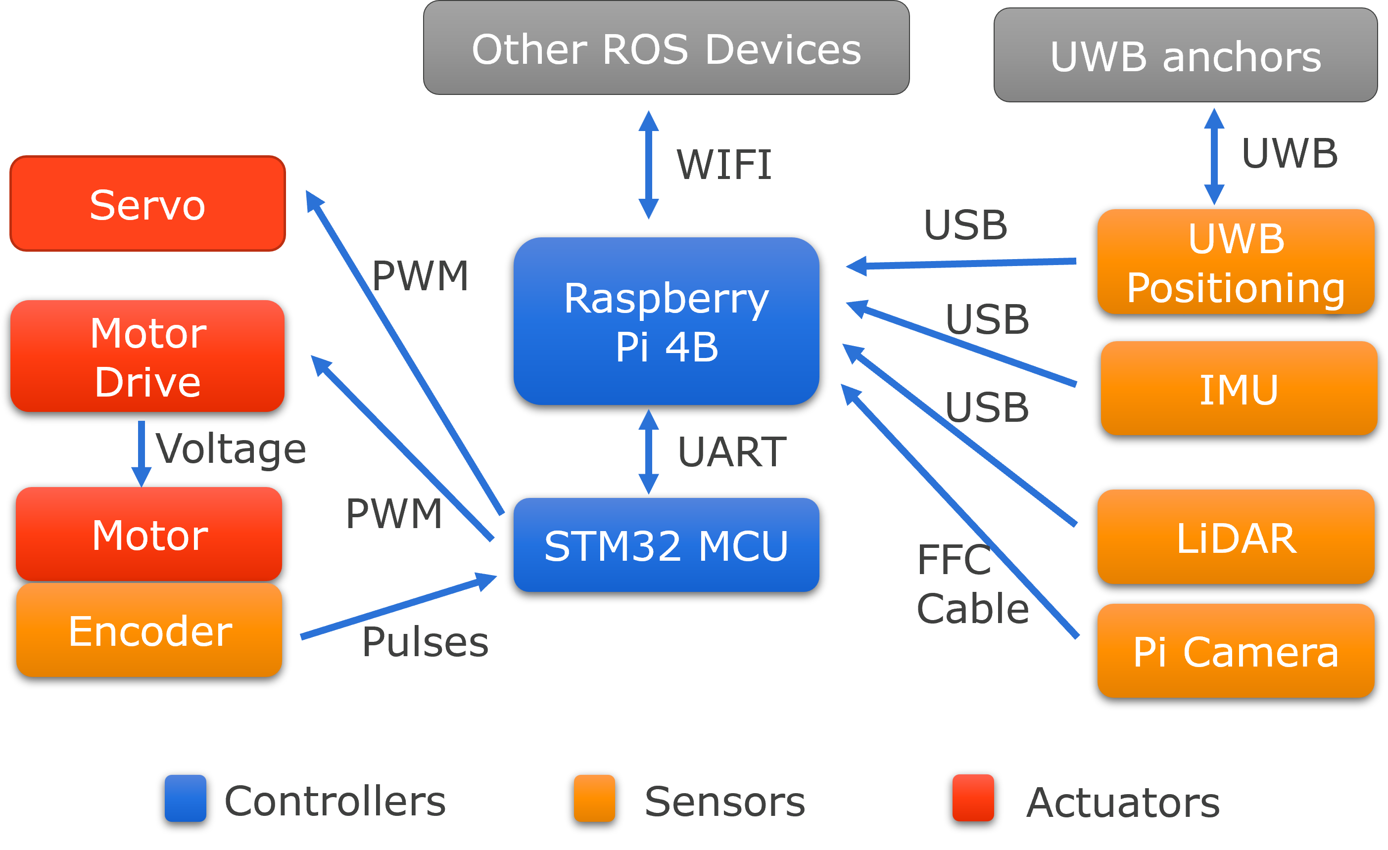
Autonomous vehicles sense states and environments, make decisions, and control mobility. Our robotic vehicle testbeds, whose hardware architecture is shown in the following figure, simulate these functions through the following stages:

1. Perception: Our testbed is equipped with an Inertial Measurement Unit (IMU), Ultra-wideband (UWB), and encoder sensors that measure attitude, position, and velocity, respectively. We can also use cameras and LiDAR to collect additional environmental data. However, these sensors are vulnerable to sensor attacks.

2. Decision Making: A Raspberry Pi with Robot Operating System (ROS2) serves as the main controller. It collects sensor data, estimates vehicle states, and generates control signals. The system uses different controllers for longitudinal and lateral control. For cruise control, a PID controller stabilizes the testbed’s velocity based on encoder feedback. For lane keeping, a Stanley Controller uses the front axle as its reference point, considering both heading error and cross-track error. We can also deploy the proposed attack detection and recovery algorithms on this system.

3. Control: An STM32 microcontroller with FreeRTOS system receives control signals from the Raspberry Pi through a Universal Asynchronous Receiver/Transmitter (UART) protocol. Running a real-time operating system, it performs time-sensitive tasks such as generating Pulse Width Modulation (PWM) signals to drive actuators.

4. Actuator: The actuator stage includes components such as motors and servos that execute vehicle movements according to control signals.

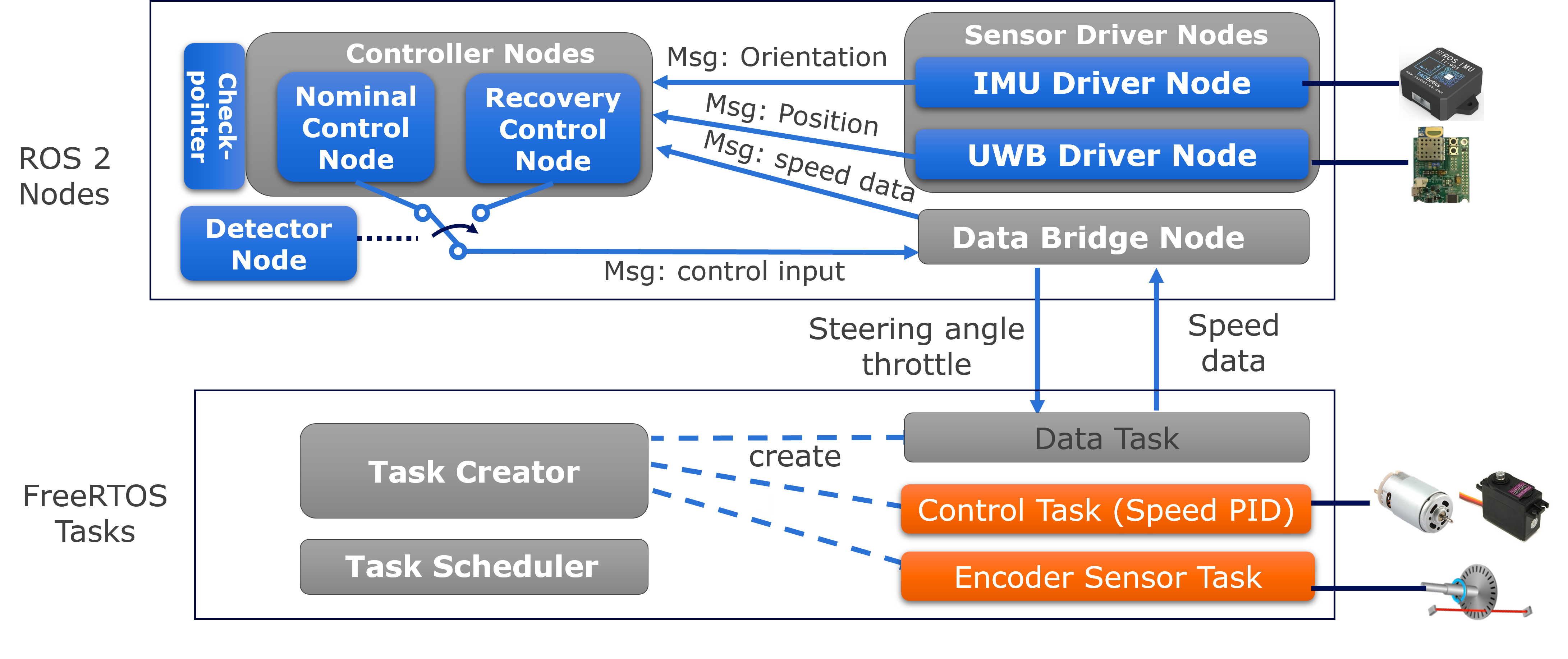
To demonstrate the toolbox usage, we show a real-time attack recovery on SVL high-fidelity simulator. We implement the LQR-based attack recovery method [2]_ on the robotic vehicle testbed, and the design is illustrated in this figure:

Autonomous vehicles perform lateral control to track paths provided by path planning modules. High-fidelity models of vehicle dynamics are complex, non-linear, and discontinuous. However, to reduce computational complexity, path tracking controllers typically consider a simplified lateral dynamics model of the vehicle (as shown in the following equation). This model approximates dynamic effects to improve tracking performance.

\begin{equation}\label{equ:lanekeeping} \frac{d}{d t} \left[\begin{array}{c} y \\ \dot{y} \\ \psi \\ \dot{\psi} \end{array}\right]=\left[\begin{array}{cccc} 0 & 1 & 0 & 0 \\ 0 & \frac{-\left(c_f+c_r\right)}{m v_x} & 0 & \frac{\left(l_r c_r-l_f c_f\right)}{m v_x}-v_x \\ 0 & 0 & 0 & 1 \\ 0 & \frac{l_r c_r-l_f c_f}{I_z v_x} & 0 & \frac{-\left(\ell_f^2 c_f+\ell_r^2 c_r\right)}{I_z v_x} \end{array}\right]\left[\begin{array}{c} y \\ \dot{y} \\ \psi \\ \dot{\psi} \end{array}\right]+\left[\begin{array}{c} 0 \\ \frac{c_f}{m} \\ 0 \\ \frac{l_f c_f}{I_z} \end{array}\right] \delta \end{equation}

Here, \(c_f\) and \(c_r\) represent cornering stiffness for the front and rear tires; \(l_f\) and \(l_r\) are the distances from the front and rear tires to the vehicle’s center of gravity; \(I_z\) is the vehicle’s moment of inertia; and \(v_x\) is the longitudinal velocity. The system states are lateral distance from the path (\(y\)), lateral error rate (\(\dot{y}\)), yaw error (\(\psi\)), and yaw error rate (\(\dot{\psi}\)). The control input is the front wheel steering angle ( \(\delta\)).

To achieve path tracking, we implement the Stanley lateral controller in ROS. The control law is expressed as \(\delta(t)=\psi(t)+\tan ^{-1}\left(\frac{k y(t)}{v_x(t)}\right)\). The yaw error (\(\psi\)) is obtained from the IMU sensor, and the lateral distance from the path (\(y\)) is obtained from the UWB sensor for indoor use. In the absence of sensor attacks, the controller can perform path tracking tasks with good performance. The attacker launches an attack on the IMU sensor, reducing the value of \(\psi\) by 0.60 radians from the start of the attack, with a detection delay of 60 control steps. Figure (a) shows the attack result as detected by the detector. Subsequently, our proposed method begins controlling the vehicle back to the safe zone, as shown in Figure (c).

Finally, we show the demonstration video here.